Note on OBI score aggregation

Introduction

The OBIC is a framework that takes a multitude of soil parameters and variables from agricultural fields and ultimately gives a single value expressing the soil quality of that field. To take this multitude of measured, modeled and calculated values to a single value between 0 and 1, three aggregation steps take place as illustrated below.

Figure 1. Graphic representation of how measured soil properties are aggregated to scores.

There is no scientific principle dictating how this aggregation should be done and there are several ways to do the aggregation. For example; averaging, linearly weighted averaging, logarithmically weighted averaging. The last one is used in OBIC. This document dives deeper into the three aggregation steps within the framework and will explain why logarithmically weighted aggregation is chosen. We will also compare the three methods of aggregation to illustrate the influence the aggregation method on the final score, which provides a kind of sensitivity analysis. The aggregation methods will be compared with a mock dataset of a selection of soil functions. Demonstration of aggregation will be performed using the dataset binnenveld. The dataset contains soil properties from 11 agricultural fields in the surroundings of Wageningen, with different soil texture and land use, and is documented in ?binnenveld.

Aggregation

Pre-processing

After calculating soil function scores and in prior to the aggregation procedure, a reformatting step takes place. The reformatting step consists of the following tasks:

it is assessed which indicators are relevant for a field given its soil type and crop category using the weight.obic table.
year numbers are assigned from 1 to n with one being the most recent year (used later for the aggregation over years)
a molten data.table is created with all indicators in a single column and soil type, crop category and year as identifying variables
indicators are assigned to categories (chemical, physical, biological, environmental, management)
the number of indicators per category is counted (used later for the aggregation over categories)
a correction factor per score is calculated based on the height of the score (used later for the aggregation within each category)
soil function scores irrelevant to the land use are set to -999

  # Step 3 Reformat dt given weighing per indicator and prepare for aggregation  ------------------
    
    # load weights.obic (set indicator to zero when not applicable)
    w <- as.data.table(OBIC::weight.obic)
    
    # Add years per field
    dt[,year := 1:.N, by = ID]
    
    # Select all indicators used for scoring
    cols <- colnames(dt)[grepl('I_C|I_B|I_P|I_E|I_M|year|crop_cat|SOILT',colnames(dt))]

    # Melt dt and assign main categories for OBI
    dt.melt <- melt(dt[,mget(cols)],
                    id.vars = c('B_SOILTYPE_AGR','crop_category','year'), 
                    variable.name = 'indicator')
    
    # add categories relevant for aggregating
    # C = chemical, P = physics, B = biological, BCS = visual soil assessment
    # indicators not used for integrating: IBCS and IM
    dt.melt[,cat := tstrsplit(indicator,'_',keep = 2)]
    dt.melt[grepl('_BCS$',indicator) & indicator != 'I_BCS', cat := 'IBCS']
    dt.melt[grepl('^I_M_',indicator), cat := 'IM']
    
    # Determine number of indicators per category
    dt.melt.ncat <- dt.melt[year==1 & !cat %in% c('IBCS','IM')][,list(ncat = .N),by='cat']
    
    # add weighing factor to indicator values
    dt.melt <- merge(dt.melt,w[,list(crop_category,indicator,weight_nonpeat,weight_peat)], 
                     by = c('crop_category','indicator'), all.x = TRUE)
    
    # calculate correction factor for indicator values (low values have more impact than high values, a factor 5)
    dt.melt[,cf := cf_ind_importance(value)]
    
    # calculate weighted value for crop category
    dt.melt[,value.w := value]
    dt.melt[grepl('veen',B_SOILTYPE_AGR) & weight_peat < 0,value.w := -999]
    dt.melt[!grepl('veen',B_SOILTYPE_AGR) & weight_nonpeat < 0,value.w := -999]

Aggregation within category

To aggregate scores, the relevant columns and rows are taken from the molten data.table.

 # Step 5 Add scores ------------------
    
    # subset dt.melt for relevant columns only
    out.score <-  dt.melt[,list(cat, year, cf, value = value.w)]
  
    # remove indicator categories that are not used for scoring
    out.score <- out.score[!cat %in% c('IBCS','IM','BCS')]

The indicators within each category are aggregated to a single score per category (chemical, physical, biological, management, environmental) using the correction factor (vcf) calculated previously using cf_ind_importance(). This correction factor vcf gives a higher weight to indicators with a lower score, as: $vcf = 1/(I+0.2)$ where I is the score of the indicator. This way, the lowest indicator, supposedly also the most limiting factor for crop production, becomes more important. Consequently, improving a low scoring indicator by 0.1 has a greater impact on the aggregated category score than improving a high scoring indicator by the same amount, making it more worthwhile to invest in the poorest and most limiting indicator.

Subsequently, the score of each category is computed by summing up the weighted values (scaled by the sum of all weights) of all soil indicators within the category: $S = \sum_{i}(I_{i} \frac{vcf_{i}}{\sum_{i}vcf_{i}})$ where S is the score of the category, vcf_i is the weighing factor of the indicator i, I_i is the score of the indicator i. This gives a single score for each of the five indicator categories (chemical, physical, biological, management, and environmental) for a specific year.

    # calculate weighted average per indicator category
    out.score <- out.score[,list(value = sum(cf * pmax(0,value) / sum(cf[value >= 0]))), by = list(cat,year)]
  
      # for case that a cat has one indicator or one year and has NA
      out.score[is.na(value), value := -999]

Aggregation over years

To account for the entire crop rotation, OBIC aggregates scores of multiple years. For the aggregation over years, another correction factor ycf is used to give more weight to recent years on a logarithmic scale. OBIC set the maximum length of period as 10 years, as crop rotation in the Netherlands are hardly ever longer than 10 years. When data older than 10 years ago is used, then those years get the same weight as 10 years ago. ycf is formulated as: $ycf = ln(12 - min(y, 10))$ where y is the length of years before the assessment. y = 1 means the year for which the assessment is conducted for (i.e. the most recent year).

This gives the correction factors for a period of eleven years as follows (from the most recent years to 11 years before):

#> 2.398 2.303 2.197 2.079 1.946 1.792 1.609 1.386 1.099 0.693 0.693

The most recent year carries about 3.5 times the weight of the tenth year. Notice that years ten and eleven have the same correction factor value, the minimum ycf value for a year is equal to that of year ten.

More priority (weight) is given to recent years because they better reflect the current situation. Additionally, changes in management or soil properties have a more visible effect on the scores in the recent years.

Aggregation of scores over years is done with the following two lines of code. This is analogue to the aggregation procedure within each category as described above (i.e. sum of weighted score, scaled by the sum of all weighing factors).

The aggregation procedure is coded in the following lines.

            
    # calculate correction factor per year; recent years are more important
    out.score[,cf := log(12 - pmin(10,year))]
  
    # calculate weighted average per indicator category per year
    out.score <- out.score[,list(value = sum(cf * pmax(0,value)/ sum(cf[value >= 0]))), by = cat]

This gives us a single score for each of the five indicator categories (chemical, physical, biological, management, and environmental), without time dimension.

Aggregation to single OBI score

The scores of five indicator categories are aggregated to a single, holistic, OBI-score. The category scores are weighed logarithmically based on the number of indicators underlying the category. The number of indicators per category was retrieved previously with the line
dt.melt.ncat <- dt.melt[year==1 & !cat %in% c('IBCS','IM')][,list(ncat = .N),by='cat'].
Now its merged with our score data.table.

      # merge out with number per category
      out.score <- merge(out.score,dt.melt.ncat, by='cat')

The correction factor for each category, ccf, are computed based on the number of indicators as:

$ccf = ln(ncat+1)$ where ncat is the number of the underlying indicators within the category. The weights for categories with 1 to 10 indicators are: 0.69, 1.1, 1.39, 1.61, 1.79, 1.95, 2.08, 2.2, 2.3, 2.4. Thus, a category based on 10 indicators affects the total score roughly 3.5 times more than a category based on 1 indicator. The idea behind giving more weight to categories with more underlying indicators sprouts from the idea that such a category is better supported by measurable data and better understood. Finally, the total OBIC score is calculated by summing up the weighted scores of 5 categories and dividing it by the sum of the weighing factors, in the same way as the other 2 aggregation steps.

This aggregation procedure is coded in the following lines.

    # calculate weighing factor depending on number of indicators
    out.score[,cf := log(ncat + 1)]
    # calculated final obi score
    out.score <- rbind(out.score[,list(cat,value)],
                       out.score[,list(cat = "T",value = sum(value * cf / sum(cf)))])

After the aggregation there is just a bit of code to format the names of the scores.

    # update element names
    out.score[,cat := paste0('S_',cat,'_OBI_A')]
    out.score[, value := round(value,3)]

Brief recap

Soil functions with low scores gain more weight than ones with high scores because these soil functions are supposed to be more limiting. This makes it more worthwhile (both in reality as for the OBI score) to invest in improving low scores
Values from recent years count more than values from long ago. Recent years are more reflective of the current situation and it becomes easier to see the effect of changes in management or soil properties in subsequent years
Categories with more underlying indicators have more weight in determining the total OBI score. This is because these indicators are better understood and supported and may also be more important.

Comparison with other aggregation methods

By now, we have some understanding of how measured soil function data are aggregated to an integral score within the current OBIC framework. So, now we can explore and reflect on some of the choices that were made in designing this aggregation process. The first choice we will reflect upon is that of the correction factors. In the OBIC framework, these are determined logarithmically but could also be determined linearly or not be used at all. Second, we will reflect on our choice of 2-step aggregation (i.e. first aggregated to categories and then aggregated to a holistic score),instead of aggregating indicators directly to a holistic score.

Data description

To reflect on alternative aggregation methods we have made a mock data.table similar to a data.table in the obic_field function just before aggregating scores. We will compare the aggregation methods with seven scenarios or treatments. The treatments are as follows:

Baseline means of all values are around 0.67
Low C values means of Chemical indicators are around 0.33, indicators in other categories are around 0.67
Low B values means of Biological indicators are around 0.33, indicators in other categories are around 0.67
One low C value one chemical indicator is set to 0, all other values are generated as in the baseline
One low B value one biological indicator is set to 0, all other values are generated as in the baseline
Recent years low mean values of the most recent five years are around 0.33, while the five years before that have mean values of around 0.67
Recent years high mean values of the most recent five years are around 0.67, while the five years before that have mean values of around 0.33

Each treatment has a 100 replicates whose soil function scores are randomly drawn from a distribution with a standard deviation of approximately 0.2. The mean of the distributions depends on the scenario. All values are in the 0 to 1 range.

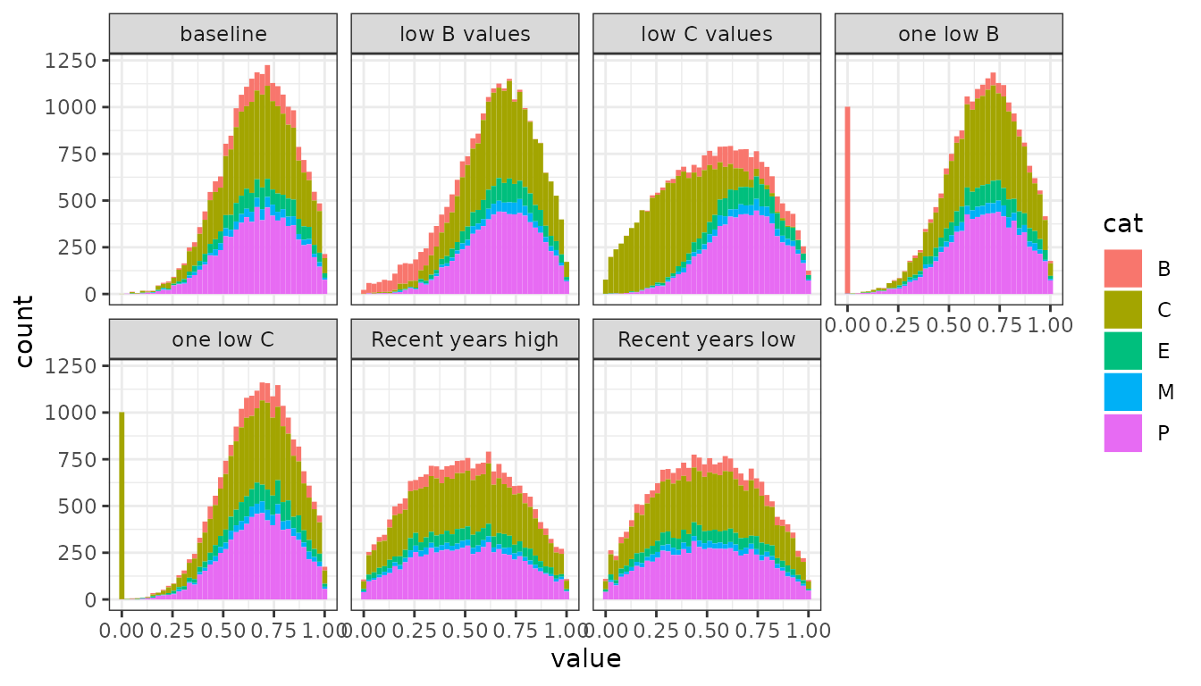
Figure 5. Distribution of indicator values per scenario as histogram

Mean scores per category for each scenario
treatment	mean B	mean C	mean E	mean M	mean P
baseline	0.672	0.671	0.671	0.670	0.673
low B values	0.328	0.670	0.676	0.678	0.676
low C values	0.675	0.328	0.674	0.666	0.671
one low B	0.335	0.674	0.672	0.667	0.673
one low C	0.670	0.596	0.674	0.680	0.675
Recent years high	0.497	0.502	0.500	0.492	0.502
Recent years low	0.504	0.500	0.495	0.501	0.502

Correction factors

To compare the influence of different correction factors, we conducted the three aggregation steps with three methods to compute a correction factor (cf):

logarithmically
linearly
no correction (averaging all values, cf = 1)

The log and linear cf’s are illustrated in Figure 2 in the range that they operate. value is the correction factor for the indicator, which ranges between 0 to 1. year is the correction factor for the year a measurement is from, 1 being the most recent year, 10 being ten years earlier. ncat is the correction for the number of soil indicators within a category. For Chemical indicators, this typically is 9. The slope of the linear correction factor is chosen such that the highest and lowest correction factor is identical between linear and logarithmic scale. In practice, another slope could be chosen for linear aggregation. The no correction method is not presented in Figure 2 as it would be a horizontal line with an arbitrary value.

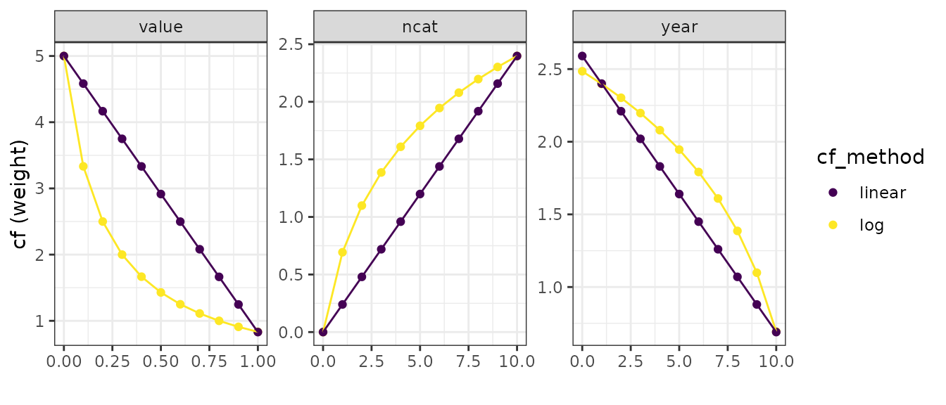
Figure 2. Correction factors calculated with linear or logarithmic methods per aggregation step.

Effects of different aggregation method on OBIC total score

The effects of different aggregation methods on total score are shown in the box plot. Red dashed lines show arithmetic means of all 22 indicators.

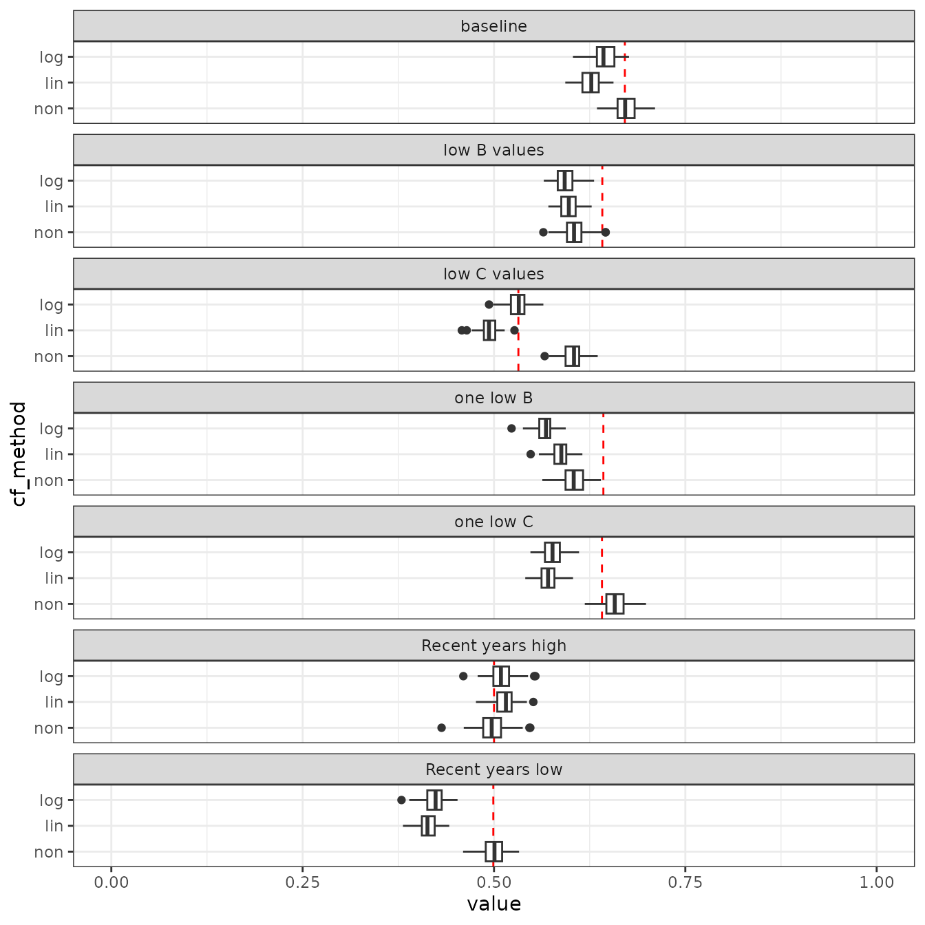
Figure 3. Total OBI score boxplots per aggregation method for each scenario.

Mean scores per category and total per aggregation method
treatment	cf_method	B	C	E	M	P	total
baseline	log	0.656	0.633	0.652	0.670	0.638	0.644
baseline	lin	0.647	0.618	0.641	0.670	0.623	0.627
baseline	non	0.672	0.671	0.671	0.670	0.673	0.671
low B values	log	0.300	0.632	0.656	0.678	0.642	0.593
low B values	lin	0.310	0.617	0.646	0.678	0.627	0.598
low B values	non	0.328	0.670	0.676	0.678	0.676	0.606
low C values	log	0.655	0.273	0.654	0.667	0.634	0.531
low C values	lin	0.645	0.295	0.644	0.667	0.619	0.493
low C values	non	0.675	0.328	0.674	0.666	0.671	0.603
one low B	log	0.123	0.637	0.655	0.666	0.638	0.566
one low B	lin	0.189	0.622	0.645	0.666	0.623	0.587
one low B	non	0.335	0.674	0.672	0.667	0.673	0.604
one low C	log	0.649	0.415	0.658	0.682	0.640	0.578
one low C	lin	0.639	0.479	0.648	0.682	0.624	0.571
one low C	non	0.670	0.596	0.674	0.680	0.675	0.659
Recent years high	log	0.518	0.501	0.521	0.535	0.503	0.510
Recent years high	lin	0.526	0.508	0.529	0.545	0.511	0.515
Recent years high	non	0.497	0.502	0.500	0.492	0.502	0.499
Recent years low	log	0.435	0.408	0.427	0.460	0.414	0.422
Recent years low	lin	0.428	0.407	0.420	0.449	0.413	0.414
Recent years low	non	0.504	0.500	0.495	0.501	0.502	0.500

In the baseline scenario, total scores are slightly lower when aggregating logarithmically or linearly compared to using no special aggregation method. In all three methods, the indicator values in the baseline are around 0.67, this number is preserved in the score when averaging all indicator values (cf_method = non) while ‘log’ and ‘lin’ scores are on average 0.03 and 0.04 lower. The change of 0.05 (in the score ranging between 0 and 1) may seem small, but it is quite large compared to the standard deviation of the distribution of the indicator values (which is 0.2). So, the difference in aggregation methods can influence the total score substantially.

The ‘lin’ and ‘log’ methods yield lower average scores because they penalize low indicator values (i.e. left-hand side in their distribution) with the weighing factor vcf. Since the ‘lin’ and ‘log’ methods were harmonised for their highest value at low indicator value (cf = 5 for value = 0), the penalty at intermediate indicator values are much higher for ‘lin’ method. This makes the average value of the OBIC score lower for ‘lin’ than ‘log’ methods. The other two aggregation steps (year aggregation (with ycf ) and category aggregation (with ccf)) causes no difference in the baseline scenario.

Note that the variation of total score is not larger for ‘lin’ and ‘log’ than ‘non’, irrespective of the larger variations in the correction factors for ‘lin’ and ‘log’. To illustrate the patterns in more details, we zoom up to the baseline scenario (Fig 4). Here we split the ‘log’ method into 4 variations: when ‘log’ method is applied for all 3 aggregation steps (‘log_all’), only for the indicator aggregation (‘log_vcf’), year aggregation (‘log_ycf’), or category aggregation (‘log_ccf’). Same applies to ‘lin’ method. Standard deviation of total score is slightly smaller when ‘log’ or ‘lin’ method is used (SD = 0.015 and 0.014, respectively) compared to when no special aggregation method is used (‘non’, SD = 0.017). Looking closer at different steps of aggregation, the variation increases due to indicator aggregation (vcf) and the year aggregation (ycf), but decreased due to category aggregation (ccf). As a result, the variation becomes smaller when linear or log method is applied to all 3 aggregation steps, largely owing to the category aggregation step. Category aggregation, irrespective of the method used for correction factor, increases variation in total score because an extreme indicator value in categories with a few indicators is strongly reflected in the total score and therefore increase the variation, compared to when total scores is directly computed from all indicators. By using ‘log’ or ‘lin’ methods in category aggregation, both of which give smaller weights to categories with a few indicators, this impact is diluted, and therefore the increase in variation becomes limited.

Figure 4. Total OBI score per aggregation method for baseline sceinario.

In the two scenario’s where one category performs poorly; ‘low B values’ and ‘low C values’, we can see the effect of using a correction factor for the number of indicators in a category. The total score in ‘low B values’ of ‘non’ method dropped by 0.065 from the baseline. This decrease is larger than the other two methods: ‘log’ and ‘lin’ dropped 0.051 and 0.029 from the baseline scenario. In contract, in scenario ‘low C values, ’log’, ‘lin’ dropped more drastically than ‘non’: the decrease in total scores was 0.113, 0.134 and 0.068 points for ‘log’, ‘lin’, and ‘non’ methods, respectively. The contrasting patterns in the change in the total score illustrate the effect of the aggregation from the 5 category scores to a single total score, which is based on the number of indicators in each category. The ‘lin’ and ‘log’ aggregation methods are more sensitive to low scores in C (a category with 9 indicators) than low scores in B (which has 2 indicators) compared to ‘non’ which is equally sensitive to a low B or C value. Furthermore, ‘log’ gives relatively heavier weight to a category with a few indicators relative to that with many indicators than ‘log’: the ratio between the weight on C and B scores is 4.5 for ‘lin’ and 2.1 for ‘log’.

The sensitivity of the scores to the number of indicators in a category is even more pronounced when looking at scenario’s ‘one low C’ and ‘one low B’, where either one chemical indicator or one biological indicator was set to 0. There is no difference between these scenario’s for the ‘non’ aggregation method, in both scenario’s a score of around 0.631 is achieved, 0.04 points lower than in the baseline. When using ‘log’ and ‘lin’ methods, scores drop 0.066 and 0.056 in one low C and 0.078 and 0.04 in one low B. Note that the drop in ‘one low B’ and ‘one low C’ scenarios compared to the baseline scenario is larger for ‘log’ than ‘lin’ method, showing that ‘log’ method is suitable for highlighting poorly-scoring indicators. In other words, ‘lin’ method imposes relatively severe penalty on moderately-scoring indicators, whereas it does not let poorly-scoring indicators stand out as much as ‘log’ method does.

The scenario’s ‘Recent years high’ and ‘Recent years low’ were included to illustrate the effect of different methods to aggregate multiple year records. In ‘Recent years low’ scenario, scores calculated with ‘lin’ and ‘log’ are substantially lower than ‘non’ method, because the lower scores in recent years gained heavier weight. In ‘Recent years high’ scenario, ‘log’ and ‘lin’ scores only slightly higher than ‘non’. Although the high recent values in ‘lin’ and ‘log’ received higher weights in the aggregation of multiple years, they are canceled out by old, low indicator values, which are severely penalized from being low.

Using correction factors, either logarithmically or linearly, can make scores more responsive to recent year, low indicator values, and categories with many underlying indicators. The magnitude of the sensitivity depends on the parameter values of the correction factors. Thus, the sensitivity presented above is merely the consequence of our current (arbitrary) choice of the parameter values, and it can be adjusted when necessary. The scores calculated with the logarithmic and linear aggregation method do not deviate largely, yet they tune the scores in slightly different ways. The difference is summarized below:

Linear aggregation method penalize intermediately-scoring indicator relatively heavily, whereas logarithmic aggregation method penalize poorly-scoring indicator heavily. If highlighting limiting soil functions is the main purpose, then logarithmic aggregation method is preferred.
Both logarithmic and linear methods intend to give heavier weight on categories with many indicators. However, the relative weight on categories with few indicators (compared to that with many indicators) are larger for logarithmic than linear methods. In other words, the contribution of a single indicator to the total score is equal for all indicators in the linear methods, whereas in the logarithmic method that is smaller for the categories with many indicators than those with a few indicators.
Both logarithmic and linear methods gives higher weight on recent years than old years. The relative weight on recent years is slightly higher for ‘lin’ than ‘log’ method, but the difference is minor.

Effects of aggregating categories on OBIC total score

Grouping indicators in categories and aggregating these categories to a single score is a choice, its not mathematically necessary. Here we look deeper at how our choice of the category aggregation influence the behavior of the OBIC score.

In the figure below, we calculated the total OBIC score both with category aggregation (‘S_T_cf_log’; with log’ method) and without category aggregation (‘S_T_nocat’; total score was calculated directly from all indicators). The other 2 aggregation steps were done with ‘log’ method for both scenarios.

When indicators of 1 category have low scores (i.e. ‘low B values’ and ‘low C values’), the total score becomes higher when the category aggregation is executed. This is because the category aggregation assures that the impact of a category on total score does not exceed a fixed proportion: the contribution of C, P, B, E and M category to the total score is 31, 30, 15, 15, 9%, respectively. When no category aggregation is done, then influence of the poor indicator values can influence the total score more prominently. When a single indicator has low scores (‘one low B’ and ‘one low C’) similar patterns were observed: the impact of the poor indicator on total score was smaller when category aggregation was one, especially in ‘one low B’ scenario.

Another advantage of using category aggregation is that it gives interpretable intermediate products of OBIC, in the form of 5 separate category scores. As shown in the previous section,the effects of the 3 aggregation steps on total score are large, and it is difficult to trace where and how the total score is influenced by different aggregation steps. In this light, computing category scores before aggregating to a total score is a nice way to provide disentangled insights to the users, allowing them to interpret different aspects of soils separately.

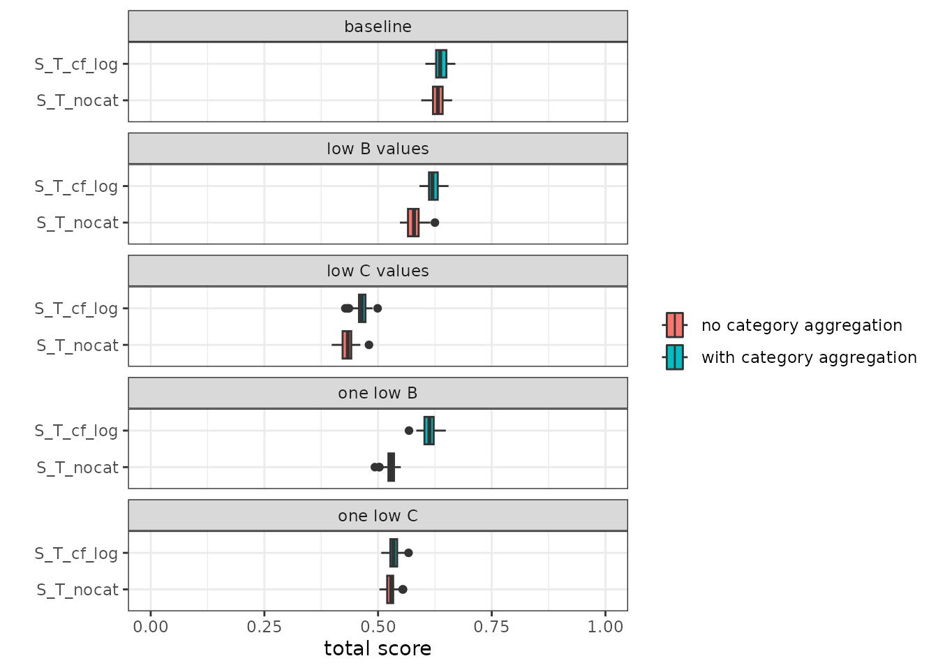
Figure 5. Scores when categories are ignored during aggregation (S_Tnocat_OBI_A) and regular aggregation (S_T_OBI_A).

Alternative aggregation methods on Binnenveld fields

The scenario’s in the experiment above use artificial data and may not be representative of actual fields in the Netherlands. Therefore we will explore the aggregation methods described above using indicator values of fields in the binnenveld dataset.

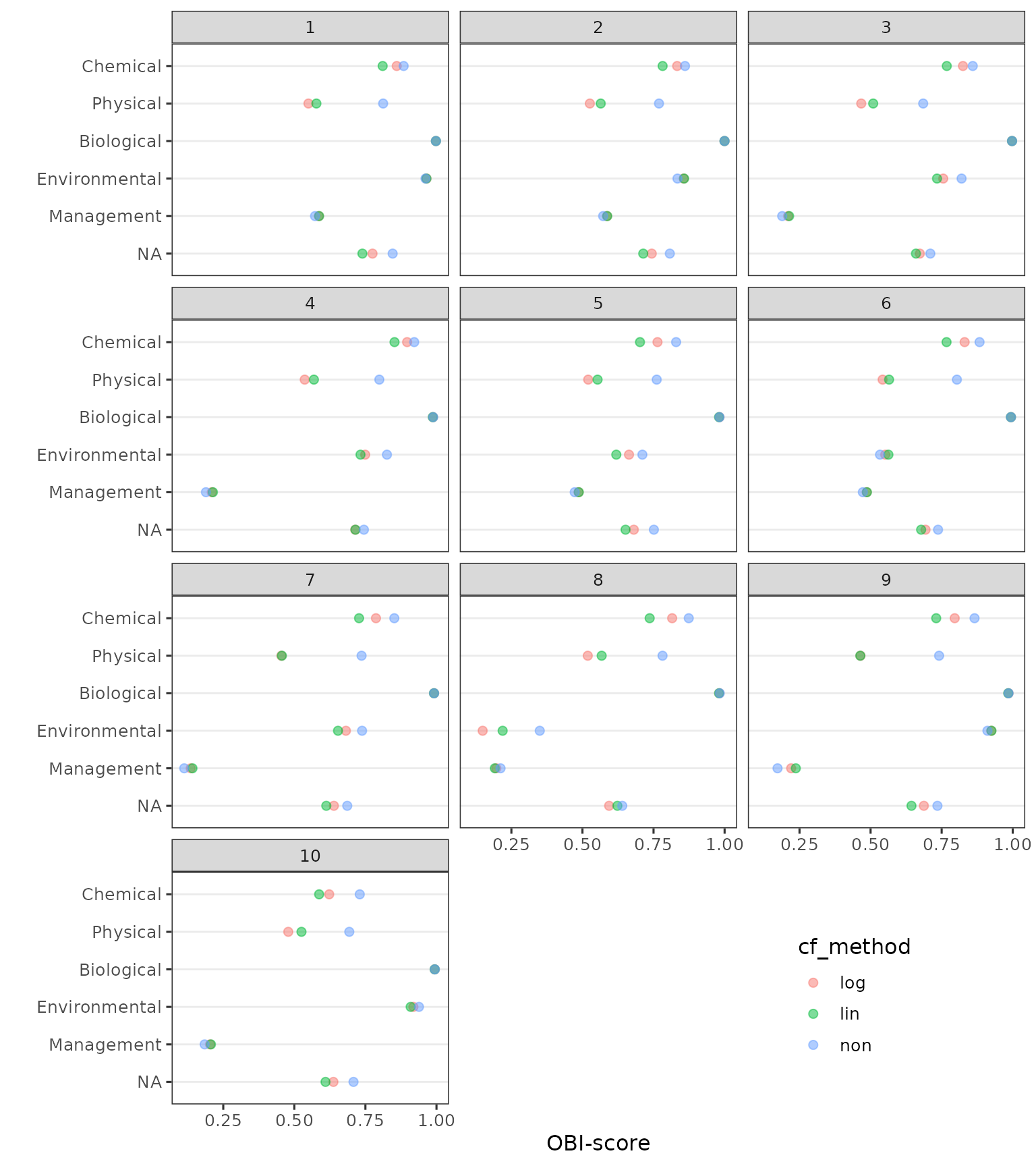
Figure 6. Total and category OBI scores of binnenveld fields aggregated with ‘log’, ‘lin’ or ‘non’ method, as well as total scores when disregarding categories in aggregating scores.

Soiltype, groundwaterclass and most frequent crop per binnenveld field.
ID	B_SOILTYPE_AGR	B_GWL_CLASS	crop_name
1	rivierklei	VI	grasland, blijvend
2	rivierklei	VI	grasland, blijvend
3	rivierklei	Vb	grasland, blijvend
4	rivierklei	VI	grasland, blijvend
5	dekzand	VII	grasland, blijvend
6	dekzand	VI	grasland, blijvend
7	dekzand	III	grasland, blijvend
8	rivierklei	VII	mais, snij-
9	dekzand	III	grasland, blijvend
10	rivierklei	V	grasland, blijvend

The binnenveld dataset lacks actual information on management parameters. In the dataset these were all set to FALSE, resulting in low management scores for all fields. For most total and categorical scores, the highest scores are obtained with the ‘non’ aggregation method and the lowest with ‘lin’.

When the aggregation step to categories is omitted, total scores differ little for some fields (eg. 2, 4, 5, 8), but are lower when using ‘log’ or ‘lin’ in other fields (eg. 3, 6, 7, 9)

Aggregation in other soil quality assessment frameworks

The OBI is not the first attempt to express soil quality with a single score, see for example: Rutgers et al. (2012) and Wijnen et al. (2012). These authors described a method to numerically express the performance of ecosystem service provision of fields with what they call: the Ecosystem Performance Index (EPX). An EPX was calculated using a set of measured properties of a field and of a reference. The reference, dubbed the Maximum Ecological Potential (MEP) was derived by selecting the best performing fields in a sample for a given land-use and soil type. Depending on the ecosystem service, a selecting of soil properties was made that acted as proxy. An EPX was calculated by comparing the selected soil properties of a field with those of the reference/MEP like this:
$EPX = 10^{-{\left(\frac{+\left|\log\left(\frac{VAR^i_{obs}}{VAR^i_{ref}}\right)\right|+\dots-\left|\log\left(\frac{VAR^{j}_{obs}}{VAR^{j}_{ref}}\right)\right|}{n}\right)}}$ Where VAR_obs is a soil property of an observed field and VAR_ref a soil property of the MEP, n is the number of distinct soil properties used to derive the EPX. Normally a variable’s contribution to the EPX is calculated using the i-type, where any deviation of the observed property from the MEP negatively affects the EPX. For some properties*ecosystem services a positive or negative deviation of the observed value from the MEP can be positive for the EPX, in such a case, the j-type has to be used. Rutgers et al. (2012) provides as example, where more soil organic matter (SOM) is always positive for providing a certain service, if an observed SOM content is higher than the reference, the j-type is used and SOM contributes negatively to the deviation from the MEP. Consequently, if the j-type is applied, the EPX of a field can be larger then one (provided that all i-type variables are at or very close to the reference). The indices of different services can be aggregated to a single score by taking the arithmetic mean. A weighted mean was also calculated based on the relative importance stakeholders assign to each service (here, a farmer, water manager and national government representative were used).

This method relies on statistical modeling for the selection of soil properties relevant for specific services rather then empirical relations. Furthermore, the reliance on BPJ for determining the reference makes the method vulnerable to the available experts and data. Both are drawbacks the authors recommend addressing.

In addition, we found that this method is sensitive to the numeric spread, values of a soil property are likely to have. When calculating natural attenuation capacity according to Wijnen et al. (2012) using observed and reference values from Rutgers et al. (2008), we found that one of the parameters FMA, had a much larger impact on the EPX than the others. Values of FMA within the 5^th and 95^th percentile ranged from 14 to 3960, while pH for example, ranged from 7.3 to 7.7

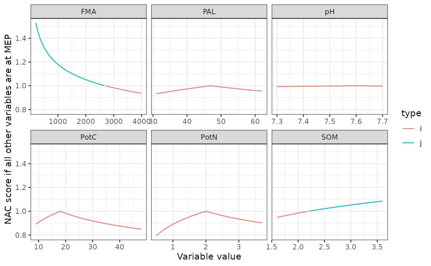
NAC scores where one variable varies and the others are set to Maximum ecological potential (MEP), variable values range from 5th percentile to 95th percentile reported by Rutgers (2008). Type indicates whether standard calculation (i) is used or not(j) where j improves on the NAC.

References

Rutgers, M, C Mulder, AJ Schouten, J Bloem, JJ Bogte, Breure AM, L Brussaard, et al. 2008. “Soil ecosystem profiling in the Netherlands with ten references for biological soil quality.” Rijksinstituut voor Volksgezondheid en Milieu RIVM. https://rivm.openrepository.com/bitstream/10029/260810/3/607604009.pdf.

Rutgers, M, H J van Wijnen, A J Schouten, C Mulder, A M P Kuiten, L Brussaard, and A M Breure. 2012. “A method to assess ecosystem services developed from soil attributes with stakeholders and data of four arable farms.” Science of The Total Environment 415: 39–48. https://doi.org/https://doi.org/10.1016/j.scitotenv.2011.04.041.

Wijnen, H J van, M Rutgers, A J Schouten, C Mulder, D de Zwart, and A M Breure. 2012. “How to calculate the spatial distribution of ecosystem services — Natural attenuation as example from The Netherlands.” Science of The Total Environment 415: 49–55. https://doi.org/https://doi.org/10.1016/j.scitotenv.2011.05.058.

Brent Riechelman, Yuki Fujita

2024-09-10